Polar Signals Continuous Profiler is compatible with any pprof formatted profile, Go deeply integrates with pprof and even supports its label feature. However, since announcing our continuous profiling product we have had many conversations with software engineers using profiling we have found that many engineers are not sure how to use them, or what effect they will have on the profiles produced. This article attempts to demystify pprof labels, using some example go code to profile.
The Basics
Pprof labels are only supported when using the CPU profiler in Go. Go's profiler is a sampling profiler, meaning at a certain frequency (by default 100 times per second) the profiler looks at the currently executing function call stack and records that. Roughly speaking, using labels, the developer can mark function call stacks to be differentiated when sampled, and only aggregated when the function call stack, as well as the labels, are identical.
Adding label instrumentation in Go is done using the `runtime/pprof` package. The most convenient way is to use the pprof.Do function.
pprof.Do(ctx, pprof.Labels("label-key", "label-value"), func(ctx context.Context) {// execute labeled code})
Diving in
To demonstrate labels we have published a repository with some example code. The content of that repository is used to guide parts of this blog post: https://github.com/polarsignals/pprof-labels-example
The example code in main.go does a large number of for-loop iterations based on a `tenant` passed into the `iterate` function. `tenant1` does 10 billion iterations, whereas `tenant2` does 1 billion iterations. It also records and writes a CPU profile to `./cpuprofile.pb.gz`.
For demonstration purposes of how pprof labels are manifested within the pprof profile, there is also `printprofile.go` that prints the function call stack of each sample as well as the sample value, and lastly the labels associated with the collected sample.
If we commented out the wrapping call, `pprof.Do`, then we would create a profile without labels instrumented. Using the printprofile.go programs, let's look at what the samples of the profile looks like without labels:
runtime.mainmain.mainmain.iteratePerTenantmain.iterate2540000000---runtime.mainmain.mainmain.iteratePerTenantmain.iterate250000000---Total: 2.79s
The unit of CPU profiles is nanoseconds, so all of these samples added up here result in a total of 2.79 seconds.
So far, so familiar. Now when adding labels to each `iterate` call using pprof the data looks different. Printing the samples of the profile taken with labels instrumented:
runtime.mainmain.mainmain.iteratePerTenantruntime/pprof.Domain.iteratePerTenant.func1main.iterate10000000---runtime.mainmain.mainmain.iteratePerTenantruntime/pprof.Domain.iteratePerTenant.func1main.iterate2540000000map[tenant:[tenant1]]---runtime.mainmain.mainmain.iteratePerTenantruntime/pprof.Domain.iteratePerTenant.func1main.iterate10000000map[tenant:[tenant1]]---runtime.mainmain.mainmain.iteratePerTenantruntime/pprof.Domain.iteratePerTenant.func1main.iterate260000000map[tenant:[tenant2]]---Total: 2.82s
Summing up all samples seen here results in a total of 2.82 seconds, however, because the call to `iterate` is labeled with each tenant using pprof labels, we are able to distinguish in the resulting data which tenant caused the large CPU usage. Now we can tell that 2.55 seconds of the total 2.82 seconds are spent whenever `tenant1` was passed.
Let's also have a look at the on-disk format of samples (and some of their metadata), just to demystify the format a bit more:
$ protoc --decode perftools.profiles.Profile --proto_path ~/src/github.com/google/pprof/proto profile.proto < cpuprofile.pb | grep -A12 "sample {"sample {location_id: 1location_id: 2location_id: 3location_id: 4location_id: 5value: 1value: 10000000}sample {location_id: 1location_id: 2location_id: 3location_id: 4location_id: 5value: 254value: 2540000000label {key: 14str: 15}}sample {location_id: 6location_id: 2location_id: 3location_id: 4location_id: 5value: 1value: 10000000label {key: 14str: 15}}sample {location_id: 1location_id: 2location_id: 3location_id: 7location_id: 5value: 26value: 260000000label {key: 14str: 16}}
What we see is that each sample is made up of IDs pointing to their location in the profile's `location` array. As well as multiple values. When inspecting the `printprofile.go` program closely, you will see that the last sample within the sample array is used. What has happened is that in reality two values have been recorded by Go's CPU profiler. The first represents the number of samples recorded representing this stack during the profiling period, and the second the nanoseconds it represents. The pprof proto definition describes that when the `default_sample_type` is unset (which it is in Go CPU profiles), then use the last samples in the index, therefore we use the nanoseconds values and not the samples. And lastly, we see the labels with their pointers into the string table of the pprof format.
Finally, having the data split by labels, we can make visualizations even more meaningful.
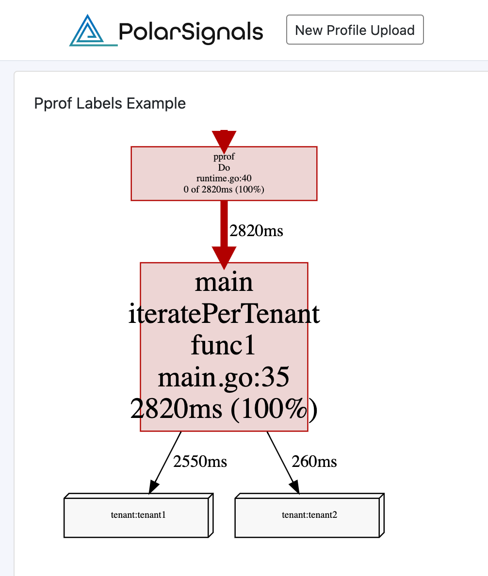
You can also explore the above profile in Polar Signals: https://share.polarsignals.com/2063c5c/
Conclusion
Pprof labels can be a great way to improve the understanding of just how different execution paths can be. We found that many people like to use them in multi-tenant systems, in order to be able to isolate performance problems that may only occur for a particular tenant in their system. As noted in the beginning, all it takes is a call to `pprof.Do`.
Polar Signals Continuous Profiler supports pprof labels in visualizations and reports! If you would like to participate in the private beta: